
As explained in Section 8, sampling is a useful technique for evaluating search strategy and the actual searches. There are several important aspects that the case team needs to consider when applying sampling for e-discovery purposes. Sampling, by its nature, produces results with certain margin of error as well as confidence measures. Therefore, the case team needs to use it carefully and consider its results in that context. Early case analysis for evaluating searches should use sample-based results as a direction to refine searches and is generally the responsibility of the case team. When sampling is used for final stages of documenting the production of ESI, the case team may need to communicate the results to the opposing team, with proper documentation of sampling parameters and sampling methodology.
This section explains various factors to consider during sampling.
A2.1. Sample Selection
A critical question is what exactly is the sample size to achieve a certain confidence level in your estimation. The theory behind sample size selection, error and confidence rates are discussed at length in statistics.[1. Statistical Sampling – Wikipedia.] [2. How to determine sample size: Six Sigma Initiative.] In some cases, the complete size of the ESI population is available to sample from, ahead of time, while in other cases the ESI population is a continuous stream of documents and we are not sure if we will have visibility into the entire population. In these cases, sampling requires selecting a document and randomly skipping a few subsequent documents in the stream. In other cases, the entire population is available, so sampling requires selecting/computing a random set of identifiable documents from the collection. Typically, one can use a pool of hash values of documents, bates number of documents and select some number of documents and only those documents are reviewed.
If your review is evaluating a single parameter for the entire collection (such as a document is Relevant vs. Not Relevant), sample size is governed by the mathematical formula:

If your desired error rate is 5% and your desired confidence level is 95%, SampleSize = 100/0.0025 = 400. Therefore, by examining one-in-four hundred documents, and determining the number of Responsive documents in that set, you can determine the actual number of relevant documents in the total population. The above formula assumes a normal distribution for the population, and the error rate measures values outside the two sigma.
Assume that the entire collection is 1,000,000 documents. Applying a requirement of 5% error rate, with 95% confidence level, you will be required to review 2,500 randomly chosen documents. Assume also that for the 2,500 documents, you determined 70 documents to be Responsive. If that were the case, you can make a statement that with 95% confidence, the total number of Responsive documents in the entire collection is in the range [26600, 29400].
Another example, this time, applying the sampling technology for measuring the Recall rate on search – let us assume that a search using Boolean logic over a set of search terms yields 5000 documents from a collection of 1,000,000 documents. One wishes to determine if the remaining 995,000 documents contain any Responsive documents. If you sample 2488 documents chosen randomly, and determine that there were 4 documents that were Responsive, you may determine that there are indeed potentially between 1520 and 1680 additional Responsive documents that could be present in the full collection. This statement again has a confidence level of 95%. As a quality improvement measure, you may examine the four documents and conduct a second search, with additional terms are specific to this query. Again, if an additional 3000 documents are selected using automated search, sampling may establish a smaller number of Responsive documents. In fact, you may increase your accuracy by selecting one in 300 documents (3,300 random documents) to get an error of 3% and confidence level of 95%. This iterative process produces a set of search terms with maximum Responsive documents.
Of course, the iterative expansion of search has the potential to retrieve larger number of documents than those that are truly responsive. In the above example, 8,000 documents were marked as Responsive by the two automated searches. If a manual review of this 8,000 documents establishes 7,500 to be truly Responsive, both your precision and recall rates are high.
In practice, the review may also be classifying documents as Privileged. For a second parameter, an independent set of sampling criteria can be established, to monitor its effectiveness.
When the underlying phenomenon is not normal distribution, one has to utilize a different formula. As an example, studies have demonstrated that the inter-arrival time of events such as customers at a coffee shop or web search hits to a web site, or the amount of time it takes to render a page are Poisson-distributed. In the case of emails in ESI, the amount of time between the sender’s submission of the message and the reply from a recipient, when viewed across all senders and recipients is also Poisson distributed.[3. Anders Johansen, Probing Human Response Times: arXiv:cond-mat/0305079v2, February 2, 2008.] [4. J.P. Eckmann, E. Moses and D. Sergi, Dialog in e-mail traffic, arXiv:cond-mat/0304433v1, February 2, 2008.] A characteristic of Poisson distribution is the long-tail distribution. However, when the time of observation is very large relative to the inter-arrival time, Poisson distribution can be approximated to a normal distribution.
As an example, if you are estimating the number of responsive documents in a five year period by examining the responsive documents in a two-week period, the Poisson λ value is approximately 260/2 or 130. For this value, Poisson approximates normal distribution.
Sampling large populations involves a random selection of n items from a large population of items, and studying a characteristic on the sample and then using the results to estimate the prevalence of that characteristic in the population. In our application of sampling, we define a population as a collection of either the set of documents that are automatically selected as responsive documents (the retrieved set), or rejected as unresponsive (unretrieved set).
Once a random sample of n documents is selected, that sample is then analyzed using human review for responsiveness. If there are documents in the sample that are truly responsive, the proportion of responsive documents in the sample is 
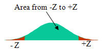
To determine these measures, the number of different ways a random selection of n items is chosen is considered. Mathematical analysis estimates confidence interval and accuracy based on the assumption that if we were to plot the proportion of responsive documents of every possible sample, that proportion follows a normal distribution. Based on this, an error in estimation is selected to be within a certain number of standard deviations. The estimate of the proportion of responsive documents from a random sample can be stated to be within a specified number of standard deviations from the sample’s proportion with a specific confidence level. The confidence level and error (based on number of standard deviations) measurements for a normal distribution are the z-score, which is a point on the normal distribution curve that encloses a certain area. For a confidence interval of 95%, the z-score is chosen so that the area under the normal distribution, between the –z and +z points total 0.95, and the area on the tails totals 0.05 of the graph.
The following table specifies various z-values for popular confidence levels.
| Confidence Level | Area between 0 and z-score | Area in one tail (alpha/2) | z-score |
|---|---|---|---|
| 50% | 0.2500 | 0.2500 | 0.674 |
| 80% | 0.4000 | 0.1000 | 1.282 |
| 90% | 0.4500 | 0.0500 | 1.645 |
| 95% | 0.4750 | 0.0250 | 1.960 |
| 98% | 0.4900 | 0.0100 | 2.326 |
| 99% | 0.4950 | 0.0050 | 2.576 |
According to this table, to achieve a confidence level of 95% and error of 5% indicates a z-score of 1.96. Given a certain z-score, we can then determine the sample size needed to achieve that error rate, using the following formulas.
Let p be the proportion of documents in the sample of sample size n that are determined to be responsive. This proportion and the z-value are related as follows.
if 0.2 < p < 0.8
if p < 0.2 or p > 0.8

For proportions that yield values in the range 0.2 to 0.8, the number of samples so that the error is e is given by the equation:
^2 \ldots (A)")
Similarly, for proportions that yield values in the range outside 0.2 to 0.8, the sample size is given by:
}{e^2}) \ldots (B)")
One complication is that the sample size depends on the sample proportion, which has not yet been determined. To overcome this, we determine a running proportion p using sample size A. We then determine a new sample size using B using that proportion and we either increase or decrease the actual sample size. Decreasing a sample size would also mean that we stop review.
The following table specifies sample sizes for various error and confidence intervals.
| Confidence Level | Error in proportion | Number of samples |
|---|---|---|
| 50% | 0.2500 | 2 |
| 80% | 0.1000 | 41 |
| 90% | 0.0500 | 271 |
| 95% | 0.0250 | 1537 |
| 98% | 0.0100 | 13526 |
| 99% | 0.0050 | 66358 |
Two typical sampling scenarios are:
- Confidence Level of 95%, with an error of 5% on the proportion (i.e. ± 0.25) requires 1537 samples to be examined.
- Confidence Level of 99%, with an error of 1% on the proportion (i.e. ± 0.005) requires 66,358 samples to be examined.
An important observation is:
Sampling a population for a certain error and confidence interval does not depend on the size of the population.
The above result is extremely significant, since this implies that regardless of the size of the input data, we only need to examine the same number of documents to be sure that we have achieved a certain confidence level that our sample proportion is within a certain range of error.
As an example, if we have 100 million documents in the unretrieved set, we need to examine only 1537 documents to determine with 95% confidence that the number of responsive documents in the unretrieved set is within the margin of error. If we find that there are 30 documents that were responsive in the unretrieved set, we can state that we have 95% confidence that the number of responsive documents in the sampled set is between 28 and 32 (rounding up the document count on the high end, rounding down on the low end). Extending that to the 100 million population, we can determine that approximately 1,951,854 ± 97,593 are responsive in the unretrieved set.
In the case of a review where errors are expensive (such as review for privilege), 99% confidence with 1% error condition would require 66,358 samples. If we identify 200 privileged documents in such a sample, you will have 99% confidence that the number of privileged documents in the sample is between 198 and 202 privileged documents.
A2.2. Sampling Pitfalls
When utilizing sampling for either reducing the scope of collection and/or review, or for quality control, one has to be careful in the actual selection methodology used. This section illustrates some common pitfalls as a cautionary commentary.
Many of the instances of perceived failures of sampling are the result of incorrect application of sampling. As an example, the following are some failures.
- The presidential election of 2000, where exit polling based on samples did not predict the outcome.
- The election for California Governor, 1982, contested by Los Angeles Mayor, Tom Bradley
- The 2004 general election in India, based on the India Shining campaign
- The Democratic Primary Election of 2008, in New Hampshire
A2.2.1 Measurement Bias
Measurement Bias occurs when the act of sampling causes the measurement to be impacted. As an example, if police decide to sample a few drivers and estimate the average speed of drivers using the fast lane of the motorway by following the selected cars on a fast lane of a highway, the results would almost always be incorrect. This is due to the fact that most cars would slow down as soon as a police vehicle follows them.
In the realm of e-discovery, measurement bias could occur if the content of the sample is known before the sampling is done. As an example, if one were to sample for responsive documents and during the sampling stage, content is reviewed, there is potential for higher-level litigation strategy to impact the responsive documents. If a project manager has communicated the cost of reviewing responsive documents, and it is understood that responsive documents should somehow be as small as possible, that could impact your sample selection. To overcome this, the person implementing the sample selection should not be provided access to the content.
A2.2.2 Coverage Bias
Coverage Bias can occur if the samples are not representative of the population due to the methodology used. As an example, if one were to device a telephone-based polling, the coverage is restricted to those reachable by telephone. The population that does not have telephones is not part of the sample, and if that population has a significantly different composition, that would not be captured in the result. This is true if there is a special correlation such as income or poverty levels and the presence of a telephone, and the sample-based polling is to estimate the level of poverty in a population.
In e-discovery, such coverage bias occurs when large portions of ESI get excluded from based on meta-data or type of ESI. As an example, Patent Litigation may require sampling technical documents in their source form, and care should be taken to include these documents in the sample selection process.
A2.2.3 Non-Response Bias
Sampling errors may appear as a result of non-response Bias. The Indian Election of 2004 illustrates this phenomenon most dramatically. In this election, a large dejected population of voting public simply refused to answer exit polling requests, or were not literate enough to answer them. Also, this group of voters was not reachable by the mainstream media, and this group overwhelmingly voted in a way contrary to the projections from the literate voting population.
In e-discovery document review, non-response bias can occur if a large percentage of potential samples is off-limits for the sampling algorithm. As an example, if an e-discovery effort is identifying potential responsive engineering documents, and if the documents are in a document format and/or programming language that could not be sampled or understood, there could be a significant non-response Bias.
A2.2.4 Response Bia
The exit polls during election of Los Angeles Mayor Tom Bradley in 1982 indicated a response bias. These opinion polls were biased by the respondent’s unwillingness to express their racist tendencies, so they chose to respond to the opinion pollsters in a way that did not evoke or expose their internal racist beliefs. In this case, the large voting block voted for the white candidate but stated to the exit pollsters that they voted for the black candidate.
Another form of response bias occurs when the participants in the survey are provided a set of questions worded in a certain way. If the same survey is worded differently, a different outcome is predicted. Also, certain wordings evoke an emotional response, tilting majority of the respondents to a Yes or No, and certain wordings overstate or understate an impact.
A response bias during sampling for e-discovery can manifest itself if sampling is used for large scale data culling. To guard against this, the sample selection process should avoid examining the contents of the documents. Any review of documents should be postponed to a post-sampling stage. A different type of response bias occurs during review, where the instructions and questions given to the reviewers and their wording can impact categorization of the reviewed documents.
A2.2.5 Sampling Time Relevance
In several cases, the selection of sample closest to the actual event is very significant. In the Democratic Primary Election of 2008, the sampling used for poll prediction was based on samples that were at least three days old, and did not include a significant number of late-deciders. Another exit polling sampling pitfall is using the earliest exit poll samples in order to be first to predict an outcome. This causes only the early voters to be counted, and the late voters are not counted to the same proportion. Also, using exit polling counts working public and absentee balloters disproportionately.
In the context of application of Sampling for e-discovery, there could be significant time periods when there was ESI and if these time periods are not properly selected, the final predictions may be completely inaccurate. As an example, if there was a significant corporate malfeasance during a certain date range, a stratified sample that treats that date range as more relevant should be considered.
A2.2.6 Sampling Continuous Stream
If the entire ESI collection is not available, one is forced to sample a stream of documents. A fundamental assumption is that the nature of the document collection does not change mid-stream. If this is not the case, samples taken at various points in time will reflect localized variations and will not reflect the true collection. Where possible, sampling should isolate collections into various strata and apply sampling within each strata independently.